Grounded World Model:
Latent Planning with
Language Goals

What is a Grounded World Model?

World model: image goalImage-goal world models such as DINO-WM and LeWM predict future features from the current frame and candidate actions, then compare them with features of a supplied goal image. The goal does not enter the predictor. The photos are the original paper assets; feature tiles are schematic.Image goalCurrent frameActionsPredictorWorld modelGrounded world model: language goalThe current frame and candidate actions produce predicted future features. These are compared with a language goal through the frozen video-language embedding model. The goal does not enter the predictor. This is a simplified overview; feature tiles are schematic.Language goalCurrent frameActionsPredictorPick up theobject that isused to hold,prepare, serve,and eat foodand liquids.Grounded world model

A world model helps a robot predict what different actions might do before trying them. This lets the robot compare possible outcomes. Methods such as DINO-WM and LeWM specify that goal with a picture of the desired result (left). The robot predicts what each action would lead to and chooses actions that bring the scene closer to the example it was given. For a new task, getting that picture may mean setting up the desired result in advance. We want to describe the goal with an ordinary instruction instead (right), such as asking the robot to pick up an object used to serve food. With GWM, the planner compares predicted outcomes with what we asked for, letting us give new goals in words without a goal picture.

How to build a Grounded World Model

We start with a video-language embedding model that connects videos with language. Keeping it frozen, we train a predictor to imagine action outcomes in its latent representation. The robot can then compare possible futures with a language goal before acting.

A Video-Language Embedding Model as the Foundation

Which trajectory matches the text?Three Isaac Sim recordings show the robot picking up a bowl, picking up a banana, or opening a blue cabinet drawer. Matching-color arrows extend from the videos into a frozen vision encoder and then a frozen backbone, followed by three embedding vectors. The text goal “Pick up the bowl” then fades in and enters the backbone directly. The text vector appears closest in direction to trajectory A, the bowl grasp. All vectors share an origin and length. Directions are a conceptual illustration.FrozenVision encoderFrozenBackboneText goal“Pick up the bowl.”Embedding spaceABCText
A · Pick up a bowl
B · Pick up a banana
C · Open a drawer

A video-language embedding model can find videos that match a description, or rank videos by how well they express the goal. It represents videos and text as vectors in a shared space, where similar directions indicate similar meaning. This allows us to describe an action, an object, or a desired outcome in words and compare it with what happens in a video.

Building GWM on the Frozen video-language embedding model

Learn from recorded futures

Given the current frame and rendered robot poses, the predictor learns to match the visual features of the recorded future using an MSE loss. The vision encoder stays frozen, and only the predictor learns. Training uses videos and actions, without task-language labels.

Learn from recorded futuresThe current frame and robot-only action renders enter a frozen vision encoder and a trainable predictor. Its predicted visual features are matched to a recorded video encoded with the same frozen weights. The token-level MSE loss updates only the predictor. The dashed GWM boundary contains the upper encoder and predictor. Frame images are original paper assets. Feature colors and convergence are schematic.Current frame + Rendered actions+GWMFrozenVision encoderTrainablePredictorPredicted featuresRecorded videoFrozenSame encoderActual future featuresMSE lossOnly the predictor learns

Planning with GWM in Latent Space

Keeping the current frame fixed, GWM predicts futures for many candidate action sequences. The same predicted futures can be compared with different language goals. Changing the task description changes each candidate’s cosine cost, reshaping the cost landscape and which action the planner prefers. No goal image or task-specific demonstrations are needed.

The same predicted futures, different language goalsOne current frame is shared by three separate candidate action sequences: A grasps a bowl, B grasps a banana, and C opens a blue cabinet drawer. All robot-only render panels retain the full camera view on a consistent light presentation background. The ellipsis represents more possible candidates. GWM predicts visual features independently of the language goal. The frozen backbone produces fixed future embeddings A, B and C. Selecting a prompt changes only its goal embedding and the corresponding cosine cost over the same action space. Future-vector angles and candidate action coordinates stay fixed. The cost landscape is one minus cosine similarity in an illustrative two-dimensional action-parameter slice, not embedding coordinates or measured GWM outputs. Each prompt sends a black signal through the backbone into the embedding panel, reveals its goal vector, and then updates the cost field. Reduced motion shows the complete selected result immediately. The prompts cycle every seven seconds while visible, unless reduced motion is requested or a prompt is selected manually.Currentframe+Rendered action sequencesABC⋮TrainedGWMFuture featuresFrozenBackboneEmbedding spaceABCLanguage goalCost landscapecost = 1 − cosine(future, language goal)“Pick up the bowl.”ABCAction space · darker = lower cost

We use Qwen3-VL-Embedding as the frozen base model and train GWM on DROID and MolmoB0T data. No demonstrations are collected for any target task.

Watching language guide the search

We use pointing and pushing to characterize two properties of GWM-guided action generation: robust semantic grounding and fine-grained spatial precision. Pointing tests whether the search identifies the image named in an instruction. Pushing tests whether it selects trajectories that make precise contact with the named cube.

Point at the named image

Scoring camera view

Point at the dog

CEM search: point at the image of the dogA replay of 5 CEM iterations. Faint blue ticks are sampled endpoints, orange ticks are elite endpoints. Samples fade before the distribution update completes. The shaded region shows relative Gaussian density, with contours at one and two standard deviations. The distribution is clipped to the plotted workspace without changing the recorded mean or sigma. The orange line follows the distribution mean, not robot motion. The star is the best-scoring sampled endpoint and may differ from the final mean. Darker blue indicates a higher planning score, normalized separately for this instruction. The background reuses the paper's color ramp, contrast and bicubic display interpolation of the original two-centimeter grid. Pointing extends edge colors to the border; pushing feathers display colors into unmeasured boundary cells. These display treatments do not add measurements. Recorded means and spreads are smoothly interpolated between iterations. Pointing samples are recorded; pushing samples are reconstructed from the original seeds and validated against every saved iteration.Initial distribution1 / 5 · Sample1 / 5 · Keep the best1 / 5 · Refine2 / 5 · Sample2 / 5 · Keep the best2 / 5 · Refine3 / 5 · Sample3 / 5 · Keep the best3 / 5 · Refine4 / 5 · Sample4 / 5 · Keep the best4 / 5 · Refine5 / 5 · Sample5 / 5 · Keep the best5 / 5 · RefineSelected endpoint

Point at the panda

CEM search: point at the image of the pandaA replay of 5 CEM iterations. Faint blue ticks are sampled endpoints, orange ticks are elite endpoints. Samples fade before the distribution update completes. The shaded region shows relative Gaussian density, with contours at one and two standard deviations. The distribution is clipped to the plotted workspace without changing the recorded mean or sigma. The orange line follows the distribution mean, not robot motion. The star is the best-scoring sampled endpoint and may differ from the final mean. Darker blue indicates a higher planning score, normalized separately for this instruction. The background reuses the paper's color ramp, contrast and bicubic display interpolation of the original two-centimeter grid. Pointing extends edge colors to the border; pushing feathers display colors into unmeasured boundary cells. These display treatments do not add measurements. Recorded means and spreads are smoothly interpolated between iterations. Pointing samples are recorded; pushing samples are reconstructed from the original seeds and validated against every saved iteration.Initial distribution1 / 5 · Sample1 / 5 · Keep the best1 / 5 · Refine2 / 5 · Sample2 / 5 · Keep the best2 / 5 · Refine3 / 5 · Sample3 / 5 · Keep the best3 / 5 · Refine4 / 5 · Sample4 / 5 · Keep the best4 / 5 · Refine5 / 5 · Sample5 / 5 · Keep the best5 / 5 · RefineSelected endpoint

Point at the banana

CEM search: point at the image of the bananaA replay of 5 CEM iterations. Faint blue ticks are sampled endpoints, orange ticks are elite endpoints. Samples fade before the distribution update completes. The shaded region shows relative Gaussian density, with contours at one and two standard deviations. The distribution is clipped to the plotted workspace without changing the recorded mean or sigma. The orange line follows the distribution mean, not robot motion. The star is the best-scoring sampled endpoint and may differ from the final mean. Darker blue indicates a higher planning score, normalized separately for this instruction. The background reuses the paper's color ramp, contrast and bicubic display interpolation of the original two-centimeter grid. Pointing extends edge colors to the border; pushing feathers display colors into unmeasured boundary cells. These display treatments do not add measurements. Recorded means and spreads are smoothly interpolated between iterations. Pointing samples are recorded; pushing samples are reconstructed from the original seeds and validated against every saved iteration.Initial distribution1 / 5 · Sample1 / 5 · Keep the best1 / 5 · Refine2 / 5 · Sample2 / 5 · Keep the best2 / 5 · Refine3 / 5 · Sample3 / 5 · Keep the best3 / 5 · Refine4 / 5 · Sample4 / 5 · Keep the best4 / 5 · Refine5 / 5 · Sample5 / 5 · Keep the best5 / 5 · RefineSelected endpoint

Point at the strawberry

CEM search: point at the image of the strawberryA replay of 5 CEM iterations. Faint blue ticks are sampled endpoints, orange ticks are elite endpoints. Samples fade before the distribution update completes. The shaded region shows relative Gaussian density, with contours at one and two standard deviations. The distribution is clipped to the plotted workspace without changing the recorded mean or sigma. The orange line follows the distribution mean, not robot motion. The star is the best-scoring sampled endpoint and may differ from the final mean. Darker blue indicates a higher planning score, normalized separately for this instruction. The background reuses the paper's color ramp, contrast and bicubic display interpolation of the original two-centimeter grid. Pointing extends edge colors to the border; pushing feathers display colors into unmeasured boundary cells. These display treatments do not add measurements. Recorded means and spreads are smoothly interpolated between iterations. Pointing samples are recorded; pushing samples are reconstructed from the original seeds and validated against every saved iteration.Initial distribution1 / 5 · Sample1 / 5 · Keep the best1 / 5 · Refine2 / 5 · Sample2 / 5 · Keep the best2 / 5 · Refine3 / 5 · Sample3 / 5 · Keep the best3 / 5 · Refine4 / 5 · Sample4 / 5 · Keep the best4 / 5 · Refine5 / 5 · Sample5 / 5 · Keep the best5 / 5 · RefineSelected endpoint
SamplesElite samplesSampling GaussianMean pathSelected endpoint

The robot searches for a position above the photo named by the instruction. Each round samples possible endpoints, scores their predicted outcomes with GWM, and shifts the next round toward the best candidates. The selected endpoint lies inside the named photo’s cell in all four searches.

Push the named cube

Scoring camera view

Push the red cube

CEM search: push the red cubeA replay of 4 CEM iterations. Faint blue ticks are sampled endpoints, orange ticks are elite endpoints. Samples fade before the distribution update completes. The shaded region shows relative Gaussian density, with contours at one and two standard deviations. The distribution is clipped to the plotted workspace without changing the recorded mean or sigma. The orange line follows the distribution mean, not robot motion. The star is the best-scoring sampled endpoint and may differ from the final mean. Darker blue indicates a higher planning score, normalized separately for this instruction. The background reuses the paper's color ramp, contrast and bicubic display interpolation of the original two-centimeter grid. Pointing extends edge colors to the border; pushing feathers display colors into unmeasured boundary cells. These display treatments do not add measurements. Recorded means and spreads are smoothly interpolated between iterations. Pointing samples are recorded; pushing samples are reconstructed from the original seeds and validated against every saved iteration.Initial distribution1 / 4 · Sample1 / 4 · Keep the best1 / 4 · Refine2 / 4 · Sample2 / 4 · Keep the best2 / 4 · Refine3 / 4 · Sample3 / 4 · Keep the best3 / 4 · Refine4 / 4 · Sample4 / 4 · Keep the best4 / 4 · RefineSelected endpoint

Push the green cube

CEM search: push the green cubeA replay of 4 CEM iterations. Faint blue ticks are sampled endpoints, orange ticks are elite endpoints. Samples fade before the distribution update completes. The shaded region shows relative Gaussian density, with contours at one and two standard deviations. The distribution is clipped to the plotted workspace without changing the recorded mean or sigma. The orange line follows the distribution mean, not robot motion. The star is the best-scoring sampled endpoint and may differ from the final mean. Darker blue indicates a higher planning score, normalized separately for this instruction. The background reuses the paper's color ramp, contrast and bicubic display interpolation of the original two-centimeter grid. Pointing extends edge colors to the border; pushing feathers display colors into unmeasured boundary cells. These display treatments do not add measurements. Recorded means and spreads are smoothly interpolated between iterations. Pointing samples are recorded; pushing samples are reconstructed from the original seeds and validated against every saved iteration.Initial distribution1 / 4 · Sample1 / 4 · Keep the best1 / 4 · Refine2 / 4 · Sample2 / 4 · Keep the best2 / 4 · Refine3 / 4 · Sample3 / 4 · Keep the best3 / 4 · Refine4 / 4 · Sample4 / 4 · Keep the best4 / 4 · RefineSelected endpoint

Push the blue cube

CEM search: push the blue cubeA replay of 4 CEM iterations. Faint blue ticks are sampled endpoints, orange ticks are elite endpoints. Samples fade before the distribution update completes. The shaded region shows relative Gaussian density, with contours at one and two standard deviations. The distribution is clipped to the plotted workspace without changing the recorded mean or sigma. The orange line follows the distribution mean, not robot motion. The star is the best-scoring sampled endpoint and may differ from the final mean. Darker blue indicates a higher planning score, normalized separately for this instruction. The background reuses the paper's color ramp, contrast and bicubic display interpolation of the original two-centimeter grid. Pointing extends edge colors to the border; pushing feathers display colors into unmeasured boundary cells. These display treatments do not add measurements. Recorded means and spreads are smoothly interpolated between iterations. Pointing samples are recorded; pushing samples are reconstructed from the original seeds and validated against every saved iteration.Initial distribution1 / 4 · Sample1 / 4 · Keep the best1 / 4 · Refine2 / 4 · Sample2 / 4 · Keep the best2 / 4 · Refine3 / 4 · Sample3 / 4 · Keep the best3 / 4 · Refine4 / 4 · Sample4 / 4 · Keep the best4 / 4 · RefineSelected endpoint

Where the cubes end up

SamplesElite samplesSampling GaussianMean pathSelected endpoint

Each endpoint defines a straight gripper slide. The search narrows toward the named cube, but reaching that region does not guarantee a push. Across 300 executed searches, 153 move the target by at least 3 cm, and none move an unnamed cube.

From Isaac Sim to the real world

For richer manipulation, we combine the GWM cost with language-blind trajectory proposals and geometric motion planning. Experiments in Isaac Sim and on a Franka robot test instructions that refer to objects, functions, and spatial relationships.

In Isaac Sim

The simulated tabletop setting includes 14 tasks with five trials each. GWM retains some ability to reason about spatial relations, visual attributes, and object affordances when deciding what the robot should pick up or where it should place an object.
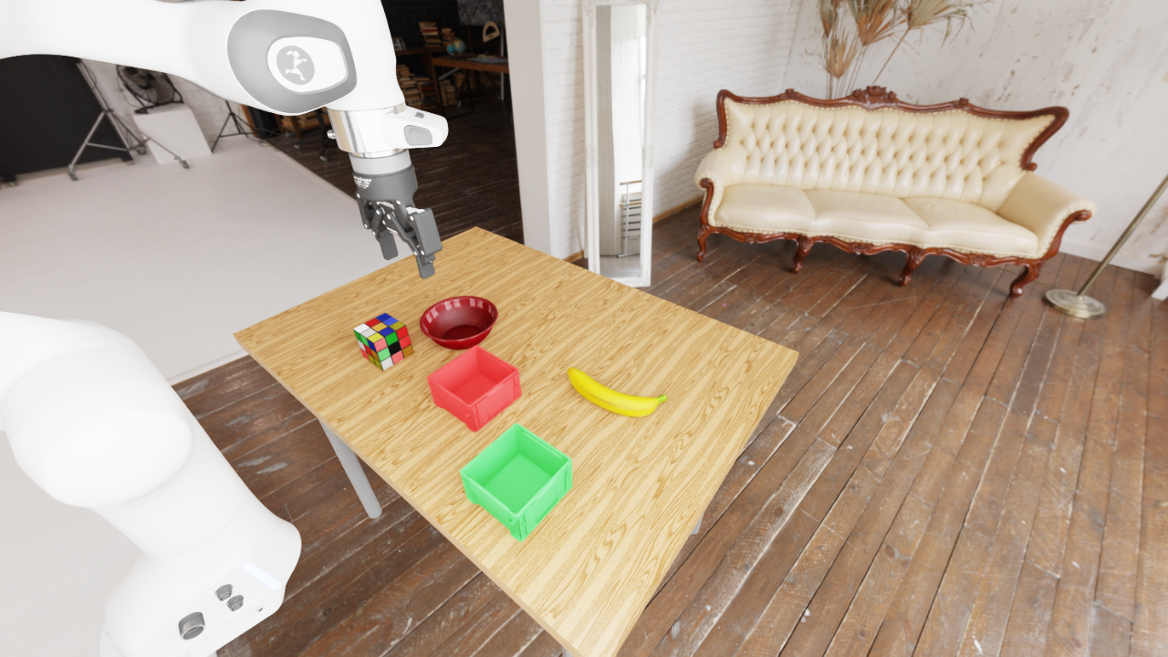
Isaac Sim scene with a Franka arm, banana, puzzle cube, red bowl, and red and green bins.

14 tasks × 5 trials. System-level success.

* π0.5 uses a relaxed pick criterion: a lift above 1 cm at any point in the episode.

† V-JEPA 2-AC is given a goal image.

Task success

Isaac Sim system-level success across 14 tasks with five trials each.
MethodSuccessRate
GWM70/70100%
GWM · opposite view65/7093%
TiPToP66/7094%
π0.5*37/7053%
V-JEPA 2-AC†25/7036%

10 Picking Tasks

  • pick up the fruit
  • pick up the yellow object
  • pick up the thing you could eat
  • pick up the object that is neither a toy nor a container
  • pick up the puzzle toy
  • pick up the most colorful object
  • pick up the object closest to the bowl that is not red
  • pick up the object you would eat a meal from
  • pick up the object between the cube and the banana
  • pick up the round container

4 Placing Tasks

  • put the block into the red box
  • put the block into the green box
  • put the block into the box that has the color of a tomato
  • put the block into the box that has the color of grass

On a real robot

The same model guides a Franka in tabletop scenes with new objects, instructions, and camera viewpoints. It retains some ability to reason about spatial relations, visual attributes, and object affordances, using language to identify objects by their appearance, location, or potential use.

55/60

Successful GWM-system sub-tasks on hardware, compared with 52/60 for TiPToP. GWM inference runs on an RTX 5090 using up to 24 GB of CUDA memory, while TiPToP relies on a frontier Gemini model.